Abstract
The impact of the closely related nature of planetary and synoptic waves is the motivation for this Solution. This Solution attempts to identify periodic upper atmospheric modes that subscribe to repeated weather occurrences.
Introduction
The recurring behavior of observed upper air patterns is reflected as future weather based on the empirical data via statistical modeling. In this pattern correlation phase space, each point represents a possible instantaneous state of the system. A solution of the governing equations is represented by a point traveling along a trajectory in the phase space. A single point in phase space determines the entire future trajectory, providing a composite of potential future weather and climate outcomes. [
1]
Background
Studies have attempted to identify recurrent modes that contribute to the alternation between active and inactive periods of subseasonal regimes. Generally, two components of variability were found to be dominant on an intraseasonal time scale: the “short-term” component, with a period of less than 1 month, and the “long-term” component, with a period of 1–2 months but apparently less than a season. Both can be referred to as the intraseasonal oscillations (ISOs) since they are clearly separated from the high-frequency synoptic-scale (less than 10 days) features and the slowly varying seasonal cycle as well. [
2]
Methods
Recurrent modes can be well observed from geopotential height (500 hPa) data. Here the method uses observations of daily 00Z 500mb from 2012 to present with a spatial resolution of 1° latitude from 45N at 10° longitude increments from 0E around the globe. Satellite observations of daily 500 hPa data provided by Navy Operational Global Atmospheric Prediction System (NOGAPS; available online at
erdNogaps1D500mb). The dataset has a spatial resolution of 1° latitude 1° longitude with global coverage. [
3]
Daily frequencies are obtained by correlating “current” patterns with “previous” patterns at lengths of 20 to 110 days for seven ~50° longitudinal wide regions. These correlation data are then reconstructed with respect to a daily top 10 for any calendar year. These daily top 10 correlations then construct a daily running average for the given calendar year (GAxA).
With the above criteria a global daily top 10 is constructed from each of the seven regions. These top 10 are then constructed into a daily running average for the given calendar year and a 15 day mode from present (M15D). Along with these frequencies, a daily average of the regional running averages is also constructed (RAxD). To overcome an evident intraseasonal jet position bias the method also seeks the top correlated frequency interval from the previous 720 days based from the present RAxD frequency (BeOP).
These frequencies (GAxA, M15D, RAxD, BeOP) are then used to seek analogs of observed wave trains and extend the encompassing weather from the present day. Deriving analog dates is accomplished by adding the forecast range to the present day then subtracting the interval rate. A three and four week forecast generated on 3/26 would provide a forecast for 4/10-23. Using an interval rate of 39, for example, would provide analog dates of 3/2-15.
Results
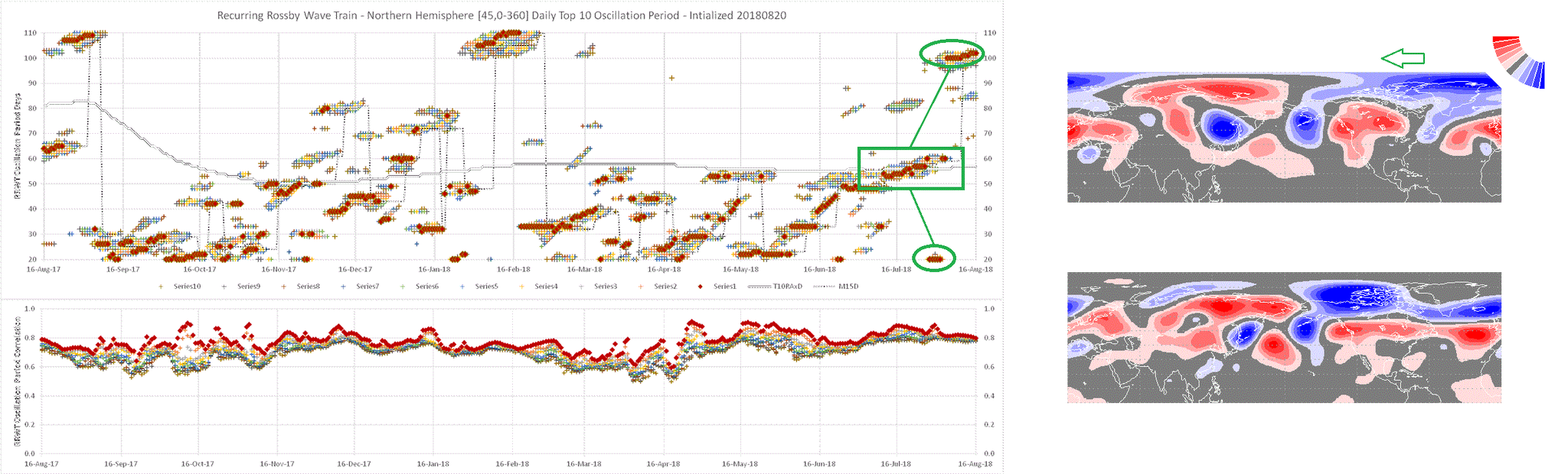
A time table displaying daily top 10 pattern correlation shows consistent features within the results. High correlated patterns centered on the 30-60 day period with top correlation greater than a 0.70 coefficient. Some interesting features are found with the time table as well. The highest coefficients form harmonious modulation of a seasonal standing wave. In addition, the 30-60 day interval displays moderate flux in correlation power with biannual dips centered on the equinox. During this time a lower frequency, interval greater than 60 days, over powers the 30-60 day interval. Also observed are periods when higher frequency, lower than a 30 day interval, are the only active intervals. [Figure 1]
Conclusions
Planetary friction and blocking will cause temporal and spatial difference in sensible weather returns. These challenges continue to advocate trial and error experiments within the framework. One theorized action incorporated a high correlated synoptic wave of 10-20 days to aid in sudden wave change. This idea proved too delicate in long range projection as it relied heavily on persistence. Another theorized action extended beyond the intraseasonal timescale and sought correlation of the average interval rate within the past two annual cycles. This idea proved robust in long range projection as it maintained a long-term longwave with seasonal sensibility.
Improvements to the framework correlation domain are desired, such as greater data points, finer grid resolution, and able mathematics. Utilization of the recurrent nature of the atmosphere can provide insight to future waveguides. The novelty of this approach is the ability to anticipate long range patterns based on recently observed patterns.
References
1. Xubin Zeng, Roger A. Pielke and R. Eykholt. Chaos Theory and Its Application to the Atmosphere. Department of Atmospheric Science, Colorado State University, Fort Collins, Colorado. 1993;74:631-44. [
Bulletin of the American Meteorological Society]
2. Bin Guan and Johnny C. L. Chan. Nonstationarity of the Intraseasonal Oscillations Associated with the Western North Pacific Summer Monsoon. Laboratory for Atmospheric Research, Department of Physics and Materials Science, City University of Hong Kong, Hong Kong, China. 2006;19:622-28. [
Bulletin of the American Meteorological Society]
3. NOGAPS 500mb data. Prior 2012 500mb data were gathered from NOAA/ESRL Radiosonde Database available online at
https://ruc.noaa.gov/raobs/.
Figure 1